Chap 8: Bayes' Rule

The multi-world perspective of statistical inference

Planet name	Appearance	Description
Earth		The planet that we care about, the place about which we want to be able to draw conclusions.
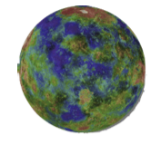
Sample		Planet Sample is populated entirely with the cases we have collected on Planet Earth. As such, it somewhat resembles Earth, but many of the details are missing, perhaps even whole countries or continents or seas. And of course, it is much smaller than Planet Earth.
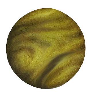
Null		Planet Null is a boring planet. Nothing is happening there. Express it how you will: All groups all have the same mean values. The model coefficients are zero. Different variables are unrelated to one another. Dullsville. But even if it’s dull, it’s not a polished billiard ball that looks the same from every perspective. It’s the clay from which Adam was created, the ashes and dust to which man returns. But it varies from place to place, and that variation is not informative. It’s just random.
Alt		This is a cartoon planet, a caricature, a simplified representation of our idea of what’s going on, our theory of how the world might be working. It’s not going to be exactly the same as Planet Earth. For one thing, our theory might be wrong. But also, no theory is going to capture all the detail and complexity of the real world.

Joke: How do you get to Planet Null? Take the Space Shuffle!

• Confidence interval: Draw many trials from Planet Sample and examine the distribution of the test statistic.
• Hypothesis testing: Draw many trials from Planet Null and examine the distribution of the test statistic.
• Power: Draw many trials from Planet Alt, conducting a Null hypothesis test on each of them, and examine the distribution of … p-values? … “significant results”?

Frequentist vs Bayesian estimation

• Classical inference is frequentist, since we are running many trials and counting how many give a particular result.
• Estimation can be either frequentist or Bayesian. They both use likelihood, the question is whether one simply maximizes likelihood or examines the likelihood times the prior.

Bayesian computations used to be hard/impossible. Now they are relatively easy.

Some proposals for “fixing science” involve switching to Bayesian packaging rather than the frequentist p-values/confidence-intervals. E.g. Bayes factors, presentation as \(\log{p}\)

Decision making

• There’s some policy choice, e.g. give a patient drug A or B, invest in real estate or the equities market, …
• There are different possible scenarios, that is, ways events may play out, each having an outcome that (generally) differs from one policy choice to another.
• We turn the possible outcomes into a score.
  • in math, called an “objective function”, in statistics, a “loss function”
• Some possible decision rules:
  • choose the policy to avoid very poor scores.
  • choose the policy that positions yourself for the best possible score
  • choose the policy that has the highest expectation value for the score

In order to employ this framework, we need both - the score function and - a probability distribution for the possible scenarios.