Users of data science are interested in two major things:
- Making predictions of (as yet) unknown variables from known variables.
- Causality: Anticipating the consequences of an intervention.
For (1), the structure of the prediction model hardly matters; it’s just the prediction error. Confidence intervals, statistical significance, etc. don’t matter.
For (2), the structure of the model matters. We want to read from the coefficients/effect-size how much influence modifying the treatment variable can have on the response.
[ADD TO BOOK, the epidemiologists’ names, e.g. treatment, effect, exposure]
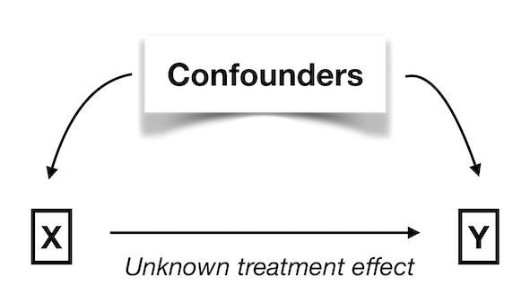
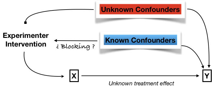
The system looks like this:
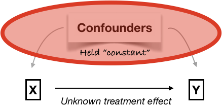
Adjustment
Unknown confounding
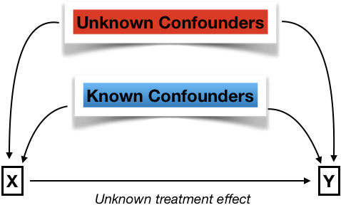
Dealing with unknown confounding
What to do …
- … when no experiment is possible?
- … when experiment will be imperfect?
- dropout
- contamination
- blunder
- broken blinding
The unknown confounders in this situaton are called lurking variables.
This leads to the often heard but hardly heeded warning: Because this was an observational study no conclusion about causality can be made.
My claim: Warnings are not sufficient. We see, from the history of p-values, how incorrect assertions can be constructed and warnings ignored.
My Proposal: The confounding interval
We need a standard process, much like the construction of a confidence interval, to illustrate the uncertainty imposed by uncontrolled confounders.
- The process cannot be based entirely on the data. By definition, the data do not tell us about the unknown factors.
- Experience and theory tells us of many situations where a claim of association was undone by a confounding variable. Extreme examples: Simpson’s paradox.
- We can likely come to a consensus about what constitutes weak, moderate, and strong confounding, even if there is no way to know which way the confounding is going.
The “plausible confounding bounds” are proposed to be a pair of multipliers on the effect size indicating the range of possibilities of how the effect size would be modified if the unknown confounders could be controlled for.
The “confounding interval” is the result of multiplying the effect size by the plausible confounding bounds.
Example:
- Suppose the difference between groups A & B was calculated to be ∆.
- Suppose the plausible confounding bounds runs from 0.5 to 1.3.
- The confounding interval will be 0.5 ∆ to 1.3 ∆
But how to come up with the plausible confounding bounds?
Some history
Jerome Cornfield considering Fisher’s proposal that a confounder, not smoking, is responsible for lung cancer and the observed correlation of smoking with cancer. Reading: Schield-1999
The question he addressed: How strong would the hypothetical confounder have to be to account entirely for the observed relationship between smoking and cancer?
In the following A = smoking, B = Fisher’s confounder. The risk ratio, r, was already known to be about 9.
If an agent, A, with no causal effect upon the risk of a disease, nevertheless, because of a positive correlation with some other causal agent, B, shows an apparent risk, r, for those exposed to A, relative to those not so exposed, then the prevalence of B, among those exposed to A, relative to the prevalence among those not so exposed, must be greater than r. – Cornfield J et al. Smoking and lung cancer: recent evidence and a discussion of some questions. JNCI 1959;22:173–203. Reprint available here.
Two approaches to the plausible confounding bounds
Troll through the historical literature looking at how known confounders change the estimate of effect size. To find this, carry out the estimation without covariates and then with covariates, translate to a ratio with/without. Collect a lot of these ratios from many study and arrange them into a distribution. Stratify the distribution by the (known) correlation between the confounders with X and Y.
Appeal to the same logic as the partial correlation coefficient, which involves working with the residuals of X on confounder C, and the residuals of Y on confounder C.
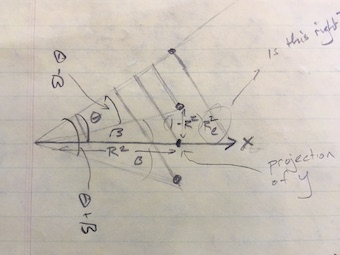
- turns into a problem in geometry, where we look at the possible distribution of C with respect to X and Y, knowing the relationship between X and Y.
There are three angles, defined by \(R^2_{xy}\). \(R^2_{xc}\), and \(R^2_{yc}\).
We know \(R^2_{xy}\) from the data. We set \(R^2_{xc}\) and \(R^2_{yc}\) in accordance with our notion of whether the uncontrolled confounding is weak, moderate, or strong.
Danny’s plausible confounding bounds
I have worked on the geometry problem to get towards a solution. I don’t know that the solution is right, but it is something that can serve as a starting point for discussion.
Known or assumed:
- values for \(R^2{xy}\), \(R^2_{xc}\), \(R^2_{yc}\).
Intermediates:
- Angle \(\theta \equiv \mbox{acos}(\sqrt{R^2_{xy}})\)
- Angle \(\beta \equiv \mbox{atan}\left( \frac{\sqrt{(1 - R^2_{xy}) R^2_{yc}}}{\sqrt{R^2_{xy}}}\right)\).
Results: The plausible confounding bounds are
- lower: \(\cos(\theta - \beta) / \cos(\theta)\) to
- upper: \(\cos(\theta + \beta) / \cos(\theta)\).
The plausible confounding bounds graphically
A proposed policy
- Did a perfect experiment? No need for plausible confounding bounds.
- Did a real experiment? Use weak plausible confounding bounds.
- Know a lot about the system you’re observing and confident that the significant confounders have been adjusted for? Use weak plausible confounding bounds.
- Not sure what all the confounders might be, but controlled for the ones you know about? Use moderate plausible confounding bounds.
- Got some data and you want to use it to figure out the relationship between X and Y? Use strong plausible confounding bounds.
## Warning in is.na(x): is.na() applied to non-(list or vector) of type
## 'expression'

## Warning in is.na(x): is.na() applied to non-(list or vector) of type
## 'expression'

## Warning in is.na(x): is.na() applied to non-(list or vector) of type
## 'expression'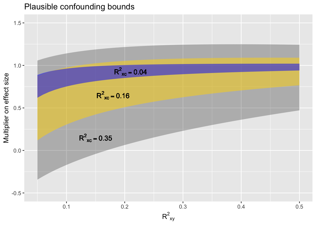
Background
A sketch of the geometry to remind Danny if someone asks where the formulas come from.